


The Keynesian Multiplier: Fiction vs. Fact
If economics was a science, the multiplier would be called (rightly) science fiction.

There are a few economic concepts that are widely cited (if not understood) by non-economists. Certainly, the “law” of supply and demand is one of them. The Keynesian (fiscal) multiplier is another; it is
the ratio of a change in national income to the change in government spending that causes it. More generally, the exogenous spending multiplier is the ratio of a change in national income to any autonomous change in spending (private investment spending, consumer spending, government spending, or spending by foreigners on the country’s exports) that causes it.
The multiplier is usually invoked by pundits and politicians who are anxious to boost government spending as a “cure” for economic downturns. What’s wrong with that? If government spends an extra $1 to employ previously unemployed resources, why won’t that $1 multiply and become $1.50, $1.60, or even $5 worth of additional output?
What’s wrong is the phony math by which the multiplier is derived, and the phony story that was long ago concocted to explain the operation of the multiplier.
MULTIPLIER MATH
To show why the math is phony, I’ll start with a derivation of the multiplier. The derivation begins with the accounting identity Y = C + I + G, which means that total output (Y) = consumption (C) + investment (I) + government spending (G). I could use a more complex identity that involves taxes, exports, and imports. But no matter; the bottom line remains the same, so I’ll keep it simple and use Y = C + I + G.
Keep in mind that the aggregates that I’m writing about here — Y , C , I , G, and later S — are supposed to represent real quantities of goods and services, not mere money. Keep in mind, also, that Y stands for gross domestic product (GDP); there is no real income unless there is output, that is, product.
Now for the derivation (right-click to enlarge this and later images):

So far, so good. Now, let’s say that b = 0.8. This means that income-earners, on average, will spend 80 percent of their additional income on consumption goods (C), while holding back (saving, S) 20 percent of their additional income. With b = 0.8, k = 1/(1 – 0.8) = 1/0.2 = 5. That is, every $1 of additional spending — let us say additional government spending (∆G) rather than investment spending (∆I) — will yield ∆Y = $5. In short, ∆Y = k(∆G), as a theoretical maximum. (Even if the multiplier were real, there are many things that would cause it to fall short of its theoretical maximum; see this, for example.)
How is it supposed to work? The initial stimulus (∆G) creates income (don’t ask how), a fraction of which (b) goes to C. That spending creates new income, a fraction of which goes to C. And so on. Thus the first round = ∆G, the second round = b(∆G), the third round = b(b)(∆G) , and so on. The sum of the “rounds” asymptotically approaches k(∆G). (What happens to S, the portion of income that isn’t spent? That’s part of the complicated phony story that I’ll examine in a future post.)
Note well, however, that the resulting ∆Y isn’t properly an increase in Y, which is an annual rate of output; rather, it’s the cumulative increase in total output over an indefinite number and duration of ever-smaller “rounds” of consumption spending.
The cumulative effect of a sustained increase in government spending might, after several years, yield a new Y — call it Y’ = Y + ∆Y. But it would do so only if ∆G persisted for several years. To put it another way, ∆Y persists only for as long as the effects of ∆G persist. The multiplier effect disappears after the “rounds” of spending that follow ∆G have played out.
The multiplier effect is therefore (at most) temporary; it vanishes after the withdrawal of the “stimulus” (∆G). The idea is that ∆Y should be temporary because a downturn will be followed by a recovery — weak or strong, later or sooner.
An aside is in order here: Proponents of big government like to trumpet the supposedly stimulating effects of G on the economy when they propose programs that would lead to permanent increases in G, holding other things constant. And other things (other government programs) are constant (at least) because they have powerful patrons and constituents, and are harder to kill than Hydra. If the proponents of big government were aware of the economically debilitating effects of G and the things that accompany it (e.g., regulations), most of them would simply defend their favorite programs all the more fiercely.
WHY MULTIPLIER MATH IS PHONY MATH
Now for my exposé of the phony math. I begin with Steven Landsburg, who borrows from the late Murray Rothbard:
. . . We start with an accounting identity, which nobody can deny:
Y = C + I + G
. . . Since all output ends up somewhere, and since households, firms and government exhaust the possibilities, this equation must be true.
Next, we notice that people tend to spend, oh, say about 80 percent of their incomes. What they spend is equal to the value of what ends up in their households, which we’ve already called C. So we have
C = .8Y
Now we use a little algebra to combine our two equations and quickly derive a new equation:
Y = 5(I+G)
That 5 is the famous Keynesian multiplier. In this case, it tells you that if you increase government spending by one dollar, then economy-wide output (and hence economy-wide income) will increase by a whopping five dollars. What a deal!
. . . [I]t was Murray Rothbard who observed that the really neat thing about this argument is that you can do exactly the same thing with any accounting identity. Let’s start with this one:
Y = L + E
Here Y is economy-wide income, L is Landsburg’s income, and E is everyone else’s income. No disputing that one.
Next we observe that everyone else’s share of the income tends to be about 99.999999% of the total. In symbols, we have:
E = .99999999 Y
Combine these two equations, do your algebra, and voila:
Y = 100,000,000
That 100,000,000 there is the soon-to-be-famous “Landsburg multiplier”. Our equation proves that if you send Landsburg a dollar, you’ll generate $100,000,000 worth of income for everyone else.
The policy implications are unmistakable. It’s just Eco 101!! [“The Landsburg Multiplier: How to Make Everyone Rich”, The Big Questions blog, June 25, 2013]
Landsburg attributes the nonsensical result to the assumption that
equations describing behavior would remain valid after a policy change. Lucas made the simple but pointed observation that this assumption is almost never justified.
. . . None of this means that you can’t write down [a] sensible Keynesian model with a multiplier; it does mean that the Eco 101 version of the Keynesian cross is not an example of such. This in turn calls into question the wisdom of the occasional pundit [Paul Krugman] who repeatedly admonishes us to be guided in our policy choices by the lessons of Eco 101. [“Multiple Comments”, op. cit,, June 26, 2013]
It’s worse than that, as Landsburg almost acknowledges when he observes (correctly) that Y = C + I + G is an accounting identity. That is to say, it isn’t a functional representation — a model — of the dynamics of the economy. Assigning a value to b (the marginal propensity to consume) — even if it’s an empirical value — doesn’t alter that fact that the derivation is nothing more than the manipulation of a non-functional relationship, that is, an accounting identity.
Consider, for example, the equation for converting temperature Celsius (C) to temperature Fahrenheit (F): F = 32 + 1.8C. It follows that an increase of 10 degrees C implies an increase of 18 degrees F. This could be expressed as ∆F/∆C = k* , where k* represents the “Celsius multiplier”. There is no mathematical difference between the derivation of the investment/government-spending multiplier (k) and the derivation of the Celsius multiplier (k*). And yet we know that the Celsius multiplier is nothing more than a tautology; it tells us nothing about how the temperature rises by 10 degrees C or 18 degrees F. It simply tells us that when the temperature rises by 10 degrees C, the equivalent rise in temperature F is 18 degrees. The rise of 10 degrees C doesn’t cause the rise of 18 degrees F.
Similarly, the Keynesian investment/government-spending multiplier simply tells us that if ∆Y = $5 trillion, and if b = 0.8, then it is a matter of mathematical necessity that ∆C = $4 trillion and ∆I + ∆G = $1 trillion. In other words, a rise in I + G of $1 trillion doesn’t cause a rise in Y of $5 trillion; rather, Y must rise by $5 trillion for C to rise by $4 trillion and I + G to rise by $1 trillion. If there’s a causal relationship between ∆G and ∆Y, the multiplier doesn’t portray it.
PHONY MATH DOESN’T EVEN ADD UP
Recall the story that’s supposed to explain how the multiplier works: The initial stimulus (∆G) creates income, a fraction of which (b) goes to C. That spending creates new income, a fraction of which goes to C. And so on. Thus the first round = ∆G, the second round = b(∆G), the third round = b(b)(∆G) , and so on. The sum of the “rounds” asymptotically approaches k(∆G). So, if b = 0.8, k = 5, and ∆G = $1 trillion, the resulting cumulative ∆Y = $5 trillion (in the limit). And it’s all in addition to the output that would have been generated in the absence of ∆G, as long as many conditions are met. Chief among them is the condition that the additional output in each round is generated by resources that had been unemployed.
In addition to the fact that the math behind the multiplier is phony, as explained above, it also yields contradictory results. If one can derive an investment/government-spending multiplier, one can also derive a “consumption multiplier”:

Taking b = 0.8, as before, the resulting value of kc is 1.25. Suppose the initial round of spending is generated by C instead of G. (I won’t bother with a story to explain it; you can easily imagine one involving underemployed factories and unemployed persons.) If ∆C = $1 trillion, shouldn’t cumulative ∆Y = $5 trillion? After all, there’s no essential difference between spending $1 trillion on a government project and $1 trillion on factory output, as long as both bursts of spending result in the employment of underemployed and unemployed resources (among other things).
But with kc = 1.25, the initial $1 trillion burst of spending (in theory) results in additional output of only $1.25 trillion. Where’s the other $3.75 trillion? Nowhere. The $5 trillion is phony. What about the $1.25 trillion? It’s phony, too. The “consumption multiplier” of 1.25 is simply the inverse of b, where b = 0.8. In other words, Y must rise by $1.25 trillion if C is to rise by $1 trillion. More phony math.
CAN AN INCREASE IN G HELP IN THE SHORT RUN?
Can an exogenous increase in G spending really yield a short-term, temporary increase in GDP? Perhaps, but there’s many a slip between cup and lip. The following example goes beyond the bare theory of the Keynesian multiplier to address several practical and theoretical shortcomings (some which are discussed “here” and “here“):
Annualized real GDP (Y) drops from $16.5 trillion a year to $14 trillion a year because of the unemployment of resources. (How that happens is a different subject.)
Government spending (G) is temporarily and quickly increased by an annual rate of $500 billion; that is, ∆G = $0.5 trillion. The idea is to restore Y to $16 trillion, given a multiplier of 5 (In standard multiplier math: ∆Y = (k)(∆G), where k = 1/(1 – MPC); k = 5, where MPC = 0.8.)
The ∆G is financed in a way that doesn’t reduce private-sector spending. (This is almost impossible, given Ricardian equivalence — the tendency of private actors to take into account the long-term, crowding-out effects of government spending as they make their own spending decisions. The closest approximation to neutrality can be attained by financing additional G through money creation, rather than additional taxes or borrowing that crowds out the financing of private-sector consumption and investment spending.)
To have the greatest leverage, ∆G must be directed so that it employs only those resources that are idle, which then acquire purchasing power that they didn’t have before. (This, too, is almost impossible, given the clumsiness of government.)
A fraction of the new purchasing power flows, through consumption spending (C), to the employment of other idle resources. That fraction is called the marginal propensity to consume (MPC), which is the rate at which the owners of idle resources spend additional income on so-called consumption goods. (As many economists have pointed out, the effect could also occur as a result of investment spending. A dollar spent is a dollar spent, and investment spending has the advantage of directly enabling economic growth, unlike consumption spending.)
A remainder goes to saving (S) and is therefore available for investment (I) in future production capacity. But S and I are ignored in the multiplier equation: One story goes like this: S doesn’t elicit I because savers hoard cash and investment is discouraged by the bleak economic outlook. Here is a more likely story: The multiplier would be infinite (and therefore embarrassingly inexplicable) if S generated an equivalent amount of I, because the marginal propensity to spend (MPS) would be equal to 1, and the multiplier equation would look like this: k = 1/(1 – MPS) = ∞, where MPS = 1.
In any event, the initial increment of C (∆C) brings forth a new “round” of production, which yields another increment of C, and so on, ad infinitum. If MPC = 0.8, then assuming away “leakage” to taxes and imports, the multiplier = k = 1/(1 – MPC), or k = 5 in this example. (The multiplier rises with MPC and reaches infinity if MPC = 1. This suggests that a very high MPC is economically beneficial, even though a very high MPC implies a very low rate of saving and therefore a very low rate of growth-producing investment.)
Given k = 5, ∆G = $0.5T would cause an eventual increase in real output of $2.5 trillion (assuming no “leakage” or offsetting reductions in private consumption and investment); that is, ∆Y = [k][∆G]= $2.5 trillion. However, because G and Y usually refer to annual rates, this result is mathematically incoherent; ∆G = $0.5 trillion does not restore Y to $16.5 trillion.
In any event, the increase in Y isn’t permanent; the multiplier effect disappears after the “rounds” resulting from ∆G have played out. If the theoretical multiplier is 5, and if transactional velocity is 4 (i.e., 4 “rounds” of spending in a year), more than half of the multiplier effect would be felt within a year from each injection of spending, and about two-thirds would be felt within two years of each injection. It seems unlikely, however, that the multiplier effect would be felt for much longer, because of changing conditions (e.g., an exogenous boost in private investment, private reemployment of resources, discouraged workers leaving the labor force, shifts in expectations about inflation and returns on investment).
All of this ignores that fact that the likely cause of the drop in Y is not insufficient “aggregate demand”, but a “credit crunch” (Michael D. Bordo and Joseph G. Haubrich in “Credit Crises, Money, and Contractions: A Historical View”, Federal Reserve Bank of Cleveland, Working Paper 09-08, September 2009). “Aggregate demand” doesn’t exist, except as an after-the-fact measurement of the money value of goods and services comprised in Y. “Aggregate demand”, in other words, is merely the sum of millions of individual transactions, the rate and total money value of which decline for specific reasons, “credit crunch” being chief among them. Given that, an exogenous increase in G is likely to yield a real increase in Y only if the increase in G leads to an increase in the money supply (as it is bound to do when the Fed, in effect, prints money to finance it). But because of cash hoarding and a bleak investment outlook, the increase in the money supply is unlikely to generate much additional economic activity.
So much for that.
THE THEORETICAL MAXIMUM
A somewhat more realistic version of multiplier math — as opposed to the version addressed earlier — yields a maximum value of k = 1:

How did I do that? In step 3, I made C a function of P (private-sector GDP) instead of Y (usually taken as the independent variable). Why? C is more closely linked to P than to Y, as an analysis of GDP statistics will prove. (Go here, download the statistics for the post-World War II era from tables 1.1.5 and 3.1, and see for yourself.)
THE TRUE MULTIPLIER
Robert J. Barro of Harvard University opens an article in The Wall Street Journal with the statement that “economists have not come up with explanations … for multipliers above one”. Barro continues:
A much more plausible starting point is a multiplier of zero. In this case, the GDP is given, and a rise in government purchases requires an equal fall in the total of other parts of GDP — consumption, investment and net exports….
What do the data show about multipliers? Because it is not easy to separate movements in government purchases from overall business fluctuations, the best evidence comes from large changes in military purchases that are driven by shifts in war and peace. A particularly good experiment is the massive expansion of U.S. defense expenditures during World War II. The usual Keynesian view is that the World War II fiscal expansion provided the stimulus that finally got us out of the Great Depression. Thus, I think that most macroeconomists would regard this case as a fair one for seeing whether a large multiplier ever exists.
I have estimated that World War II raised U.S. defense expenditures by $540 billion (1996 dollars) per year at the peak in 1943-44, amounting to 44% of real GDP. I also estimated that the war raised real GDP by $430 billion per year in 1943-44…. The other way to put this is that the war lowered components of GDP aside from military purchases. The main declines were in private investment, nonmilitary parts of government purchases, and net exports — personal consumer expenditure changed little. Wartime production siphoned off resources from other economic uses — there was a dampener, rather than a multiplier….
There are reasons to believe that the war-based multiplier of 0.8 substantially overstates the multiplier that applies to peacetime government purchases. For one thing, people would expect the added wartime outlays to be partly temporary (so that consumer demand would not fall a lot). Second, the use of the military draft in wartime has a direct, coercive effect on total employment. Finally, the U.S. economy was already growing rapidly after 1933 (aside from the 1938 recession), and it is probably unfair to ascribe all of the rapid GDP growth from 1941 to 1945 to the added military outlays. [“Government Spending Is No Free Lunch”, The Wall Street Journal, January 22, 2009]
This is from a paper by Valerie A. Ramsey:
[I]t appears that a rise in government spending does not stimulate private spending; most estimates suggest that it significantly lowers private spending. [“Government Spending and Private Activity”, National Bureau of Economic Research, January 2012]
There is a key component of government spending which usually isn’t captured in estimates of the multiplier: transfer payments, which are mainly “social benefits” (e.g., Social Security, Medicare, and Medicaid). In fact, actual government spending in the U.S., including transfer payments, is about double the nominal amount that is represented in G, the standard measure of government spending (the actual cost of government operations, buildings, equipment, etc.). But transfer payments — like other government spending — are subsidized by directing resources from persons who are directly productive (active worker) and whose investments are directly productive (innovators, entrepreneurs, stockholders, etc.) to persons who (for the most part) are economically unproductive and counterproductive. It follows that real economic output must be affected by transfer payments.
Other factors are also important to economic growth, namely, private investment in business assets, the rate at which regulations are being issued, and inflation. The combined effects of these factors and aggregate government spending have been estimated. I borrow from that estimate, with a slight, immaterial change in nomenclature:
gr = 0.0248 – 0.340F + 0.0773A -0.000336R -0.131P
Where,
gr = real rate of GDP growth in a 10-year span (annualized)
F = fraction of GDP spent by governments at all levels during the preceding 10 years [including transfer payments]
A = the constant-dollar value of private nonresidential assets (business assets) as a fraction of GDP, averaged over the preceding 10 years
R = average number of Federal Register pages, in thousands, for the preceding 10-year period
P = growth in the CPI-U during the preceding 10 years (annualized).
The r-squared of the equation is 0.74 and the F-value is 1.60E-13. The p-values of the intercept and coefficients are 0.093, 3.98E-08, 4.83E-09, 6.05E-07, and 0.0071. The standard error of the estimate is 0.0049, that is, about half a percentage point.
Given that rg = -0.340F, other things being the same, then
Y1 = Y0(c – 0.340F)
Where,
Y1 = real GDP in the period after a change in F, other things being the same
Y0 = real GDP in the period during which F changes
c = a constant, representing the sum of 1 + 0.025 + the coefficients obtained from fixed values of A, R, and P
The true F multiplier, kT, is therefore negative:
kT = ∆Y/∆F = -0.340Y0
For example, with Y0 = 1000 , F = 0 , and other things being the same,
∆Y = [1000 – (0)(1000)] = 1000, when F = 0
∆Y = [1000 – (-0.347)(1000)] = 660, when F = 1
Keeping in mind that the equation is based on an analysis of successive 10-year periods, the true F multiplier should be thought of as representing the effect of a change in the average value of F in a 10-year period on the average value of Y in a subsequent 10-year period.
This is not to minimize the deleterious effect of F (and other government-related factors) on Y. If the 1947-1957 rate of growth (4 percent) had been sustained through 2017, Y would have risen from $1.9 trillion in 1957 to $20 trillion in 2017. But because F, R, and P rose markedly over the years, the real rate of growth dropped sharply and Y reached only $17.1 trillion in 2017. That’s a difference of almost $3 trillion in a single year.
Such losses, summed over several decades, represent millions of jobs that weren’t created, significantly lower standards of living, greater burdens on the workers who support retirees and subsidize their medical care, and the loss of liberty that inevitably results when citizens are subjugated to tax collectors and regulators.
ADDENDUM: A REAL ECONOMIC EXPLANATION FOR THE INEFFECTIVENESS OF “STIMULUS” SPENDING
Consider a static, full-employment economy, in which the same goods and services are produced year after year, yielding the same incomes to the same owners of the same factors of production, which do not change in character (capital goods are maintained and replaced in kind). The owners of the factors of production spend and save their incomes in the same way year after year, so that the same goods and services are produced year after year, and those goods and services encompass the maintenance and in-kind replacement of capital goods. Further, the production cycle is such that all goods and services become available to buyers on the last day of the year, for use by the buyers during the coming year. (If that seems far-fetched, just change all instances of “year” in this post to “month”, “week”, “day”, “hour”, “minute”, or “second.” The analysis applies in every case.)
What would happen if there were a sudden alteration in this circular flow of production (supply), on the one hand, and consumption and investment (demand), on the other hand? Specifically, suppose that a component of the circular flow is a bilateral exchange between a gunsmith and a dairyman who produces butter: one rifle for ten pounds of butter. If the gunsmith decides that he no longer wants ten pounds of butter, and therefore doesn’t produce a rifle to trade for butter, the dairyman would reduce his output of butter by ten pounds.
A Keynesian would describe the situation as a drop in aggregate demand. There is no such thing as “aggregate demand”, of course; it’s just an abstraction for the level of economic activity, which really consists of a host of disparate transactions, the dollar value of which can be summed. Further, those disparate transactions represent not just demand, but demand and supply, which are two sides of the same coin.
In the case of the gunsmith and the dairyman, aggregate output drops by one rifle and ten pounds of butter. The reduction of output by one rifle is voluntary and can’t be changed by government action. The reduction of output by ten pounds of butter would be considered involuntary and subject to remediation by government – in the Keynesian view.
What can government do about the dairyman’s involuntary underemployment? Keynesians would claim that the federal government could print some money and buy the dairyman’s butter. This would not, however, result in the production of a rifle; that is, it would not restore the status quo ante. If the gunsmith has decided not to produce a rifle for reasons having nothing to do with the availability of ten pounds of butter, the government can’t change that by buying ten pounds of butter.
But, a Keynesian would say, if the government buys the ten pounds of butter, the dairyman will have money with which to buy other things, and that will stimulate the economy to produce additional goods and services worth at least as much as the rifle that’s no longer being produced. The Keynesian would have to explain how it’s possible to produce additional goods and services of any kind if only the gunsmith and dairyman are underemployed (one voluntarily, the other involuntarily). The gunsmith has declined to produce a rifle for reasons of his own, and it would be pure Keynesian presumption to assert that he could be lured into producing a rifle for newly printed money when he wouldn’t produce it for something real, namely, ten pounds of butter.
Well, what about the dairyman, who now has some newly printed money in his pocket? Surely, he can entice other economic actors to produce additional goods and services with the money, and trade those goods and services for his ten pounds of butter. The offer of newly printed money might entice some of them to divert some of their production to the dairyman, so that he would have buyers for his ten pounds of butter. Thus the dairyman might become fully employed, but the diversion of output in his direction would cause some other economic actors to be less than fully employed.
Would the newly printed money entice the entry of new producers, some combination of whom might buy the dairyman’s ten pounds of butter and restore him to full employment? It might, but so would private credit expansion in the normal course of events. The Keynesian money-printing solution would lead to additional output only where (a) private credit markets wouldn’t finance new production and (b) new production would be forthcoming despite the adverse conditions implied by (a). And the fact would remain that economic output has declined by one rifle, which fact can’t be changed by deficit spending or monetary expansion.
This gets us to the heart of the problem. Deficit spending (or expansionary monetary policy) can entice additional output only if there is involuntary underemployment, as in the case of the dairyman who would prefer to continue making and selling the ten pounds of butter that he had been selling to the gunsmith. And how do resources become involuntarily underemployed? Here are the causes, which aren’t mutually exclusive:
changes in perceived wants, tastes, and preferences, as in the case of the gunsmith’s decision to make one less rifle and forgo ten pounds of butter
reductions in output that are occasioned by forecasts of lower demand for particular goods and services
changes in perceptions of or attitudes toward risk, which reduce producers’ demand for resources, buyers’ demand for goods and services, or financiers’ willingness to extend credit to producers and buyers.
I am unaware of claims that deficit spending or monetary expansion can affect the first cause of underemployment, though there is plenty of government activity aimed at changing wants, tastes, and preferences for paternalistic reasons.
What about the second and third causes? Can government alleviate them by buying things or making more money available with which to buy things? The answer is no. What signal is sent by deficit spending or monetary expansion? This: Times are tough, demand is falling, credit is tight, In those circumstances, why would newly printed money in the pockets of buyers (e.g., the dairyman) or in the hands of banks entice additional production, purchases, lending, or borrowing?
The evidence of the Great Recession suggests strongly that printing money and spending it or placing it with banks does little if any good. The passing of the Great Recession — and of the Great Depression seventy years earlier — was owed to the eventual restoration of the confidence of buyers and sellers in the future course of the economy. In the case of the Great Depression, confidence was restored when the entry of the United States into World War II put an end to the New Deal, which actually prolonged the depression
In the case of the Great Recession, confidence was restored (though not as fully) by the end of “stimulus” spending. The lingering effort on the part of the Fed to stimulate the economy through quantitative easing probably undermined confidence rather than restoring it. In fact, the Fed announced that it would begin to raise interest rates in an effort to convince the business community that the Great Recession is really coming to an end.
ADDENDUM II: THE MULTIPLIER ACCORDING TO THE GENERAL THEORY
The essential falsity of the multiplier can be found by consulting the equation of exchange:
In monetary economics, the equation of exchange is the relation:
MV = PQ
where, for a given period,
M is the total nominal amount of money supply in circulation on average in an economy.
V is the velocity of money, that is the average frequency with which a unit of money is spent.
P is the price level.
Q is an index of real expenditures (on newly produced goods and services).
Thus PQ is the level of nominal expenditures. This equation is a rearrangement of the definition of velocity: V = PQ/M. As such, without the introduction of any assumptions, it is a tautology. The quantity theory of money adds assumptions about the money supply, the price level, and the effect of interest rates on velocity to create a theory about the causes of inflation and the effects of monetary policy.
In earlier analysis before the wide availability of the national income and product accounts, the equation of exchange was more frequently expressed in transactions form:
MVT = PT
where,
VT is the transactions velocity of money, that is the average frequency across all transactions with which a unit of money is spent (including not just expenditures on newly produced goods and services, but also purchases of used goods, financial transactions involving money, etc.).
T is an index of the real value of aggregate transactions.
(Note the careful — but easily overlooked — qualification that quantities are for “a given period”, as I have pointed out. One cannot simply add imaginary increases in real output over an unspecified span of time to an annual rate of output and obtain a new, annual rate of output.)
If the values for M, V, P, and Q are annual rates or averages, then MV = PQ = Y, the last of which I am using here to represent real GDP.
If the central government “prints” money and spends it on things (i.e., engages in deficit spending financed by the Federal Reserve’s open-market operations), then ∆G (the addition to the rate of G) = ∆M (the average annual increase in the money supply). What happens as a result of ∆M depends on the actual relationships between M and V, P, and Q. They are complex relationships, and they vary constantly with the state of economic activity and consumers’ and producers’ expectations. Even a die-hard Keynesian would admit as much.
If new economic activity (Y) is relatively insensitive to ∆G, as it is for the many reasons detailed here, it is equally insensitive to ∆M. For one thing — one very important thing — ∆M may be absorbed almost entirely by an increase in VT without a concomitant increase in Q. That is to say, ∆G necessarily implies (in the short run) an increase in transactions velocity (VT) and it is most likely to be spent on resources that are already employed (i.e, either on things that were already being produced or by displacing private purchases of things that were already being produced).
The equality MV = PQ long predates Keynes’s General Theory, in which he introduces the multiplier, and so it was well known to Keynes. As it happens, the equality is at the heart of his multiplier:
The state of the economy, according to Keynes, is determined by four parameters: the money supply, the demand functions for consumption (or equivalently for saving) and for liquidity, and the schedule of the marginal efficiency of capital determined by ‘the existing quantity of equipment’ and ‘the state of long-term expectation’ (p 246).
Adjusting the money supply is the domain of monetary policy. The effect of a change in the quantity of money is considered at p. 298. The change is effected in the first place in money units. According to Keynes’s account on p. 295, wages will not change if there is any unemployment, with the result that the money supply will change to the same extent in wage units.
We can then analyse its effect from the diagram [reproduced below], in which we see that an increase in M̂ shifts r̂ to the left, pushing Î upwards and leading to an increase in total income (and employment) whose size depends on the gradients of all 3 demand functions. If we look at the change in income as a function of the upwards shift of the schedule of the marginal efficiency of capital (blue curve), we see that as the level of investment is increased by one unit, the income must adjust so that the level of saving (red curve) is one unit greater, and hence the increase in income must be 1/S'(Y) units, i.e. k units. This is the explanation of Keynes’s multiplier.
Here’s the diagram:
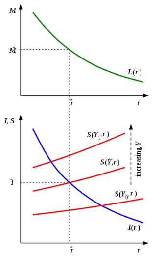
If that is the explanation of Keynes’s multiplier, it is even more backward than the usual explanation that I shredded earlier in this post. All the explanation says is that if the real money supply (M̂) is increased (i.e., not translated into higher prices) due to an exogenous increase in government spending, the real interest rate (r̂) decreases. And if the decrease in the real interest rate leads to an increase in investment, Y must rise by enough to preserve the theoretical relationship between Y and saving (S) and investment (I).
In this case, Keynes depicts the multiplier as the effect of an increase in I resulting from an increase in M, which is really an increase in G (∆G) under the condition of less than full employment (whatever that is). The increase in I is made possible by the decrease in the real rate of interest.
That’s odd, because the popular view of the multiplier is that it is the rise in real GDP that is directly attributable to a rise in government spending. Will the real multiplier please stand up?
Regardless, the relationship between the increase in I and the increase in Y is no less tautologous than it is in the usual explanation of the multiplier.Simply put, the increase in I is the increase that must result if Y increases, given an ex-post relationship between I and Y. There is no causality, except in the imagination of the proponent of increased government spending.
We are back to where we started, with a mythical multiplier that explains nothing.